Data Overview

# Read the CSV file
results <- read.csv("eurojackpot_results.csv", stringsAsFactors = FALSE)

# Convert date format to day, month, year
results$draw_date <- as.Date(results$draw_date)
results$day <- format(results$draw_date, "%d")
results$month <- format(results$draw_date, "%m")
results$year <- format(results$draw_date, "%Y")

# Split main numbers into separate columns
main_numbers_split <- strsplit(gsub("\"", "", results$main_numbers), ",")
main_numbers_matrix <- do.call(rbind, main_numbers_split)
colnames(main_numbers_matrix) <- paste0("main_", 1:5)
results <- cbind(results, main_numbers_matrix)

# Split euro numbers into separate columns
euro_numbers_split <- strsplit(gsub("\"", "", results$euro_numbers), ",")
euro_numbers_matrix <- do.call(rbind, euro_numbers_split)
colnames(euro_numbers_matrix) <- paste0("euro_", 1:2)
results <- cbind(results, euro_numbers_matrix)

# Convert number columns to numeric
for (col in c(paste0("main_", 1:5), paste0("euro_", 1:2))) {
    results[[col]] <- as.numeric(results[[col]])
}

n <- nrow(results)

Before hunting for patterns, meet the raw material. The dataset is beautifully simple: one row per draw — a date, five main numbers, two euro numbers — stretching back to the very first Eurojackpot draw in March 2012. That’s it. Everything on this site is squeezed out of those three columns.

The Dataset at a Glance

summary_df <- data.frame(
    Metric = c("Total number of draws", "Date range", "Number of years covered", "Balls drawn in total"),
    Value = c(
        format(n, big.mark = ","),
        paste(format(min(results$draw_date), "%b %d, %Y"), "to", format(max(results$draw_date), "%b %d, %Y")),
        length(unique(results$year)),
        format(n * 7, big.mark = ",")
    )
)

knitr::kable(summary_df,
    caption = "Dataset summary",
    col.names = c("Metric", "Value"),
    align = c("l", "l")
)

Dataset summary
Metric	Value
Total number of draws	828
Date range	Mar 23, 2012 to Feb 25, 2025
Number of years covered	14
Balls drawn in total	5,796

yearly <- results %>% count(year)

ggplot(yearly, aes(x = year, y = n)) +
    geom_col(fill = ej_blue, width = 0.72) +
    geom_text(aes(label = n), vjust = -0.55, size = 3.2, color = ej_ink2, fontface = "bold") +
    scale_y_continuous(expand = expansion(mult = c(0, 0.12))) +
    labs(
        title = "Number of Draws per Year",
        subtitle = "The count doubled in 2022, when Tuesday draws joined the traditional Friday draw",
        x = NULL, y = "Draws", caption = ej_caption
    ) +
    theme(panel.grid.major.x = element_blank())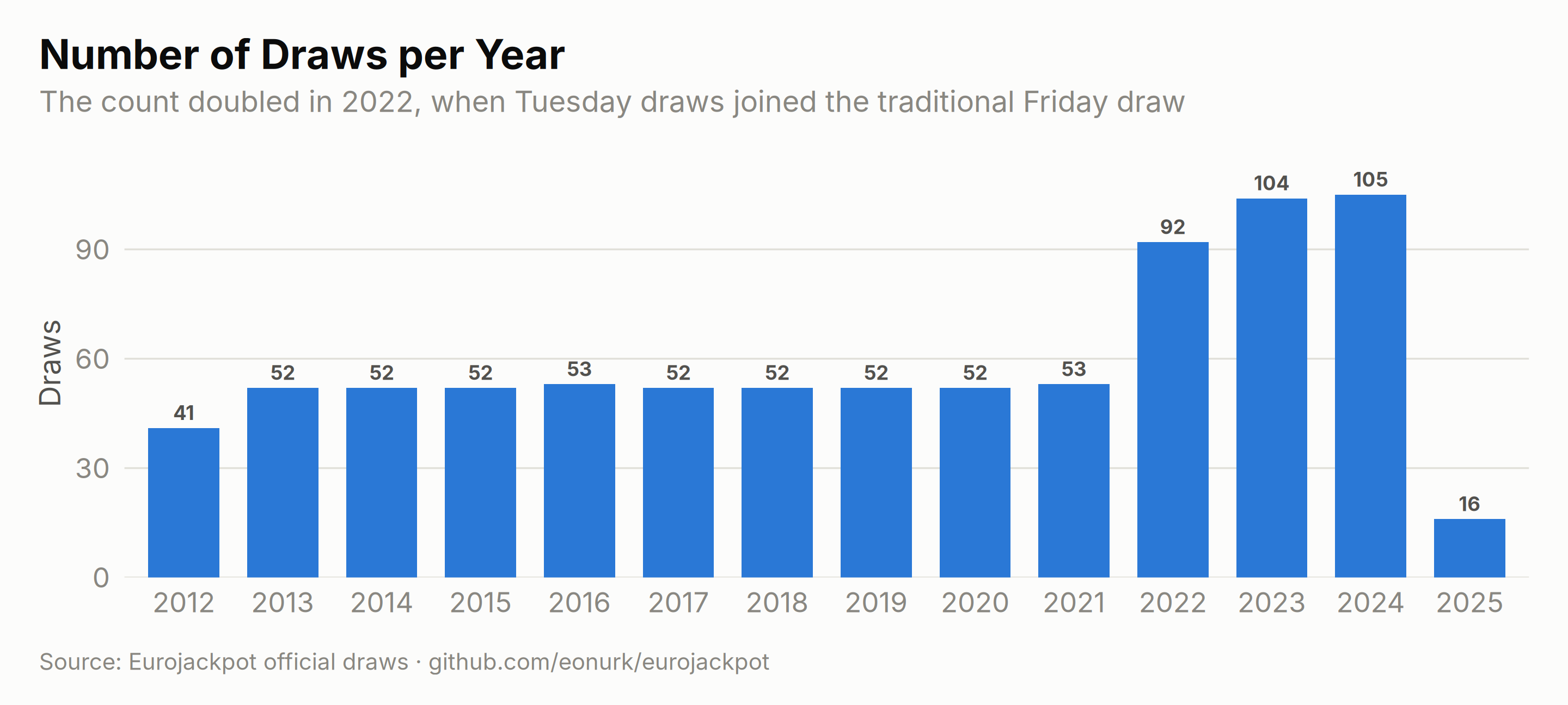

Number Frequency Analysis

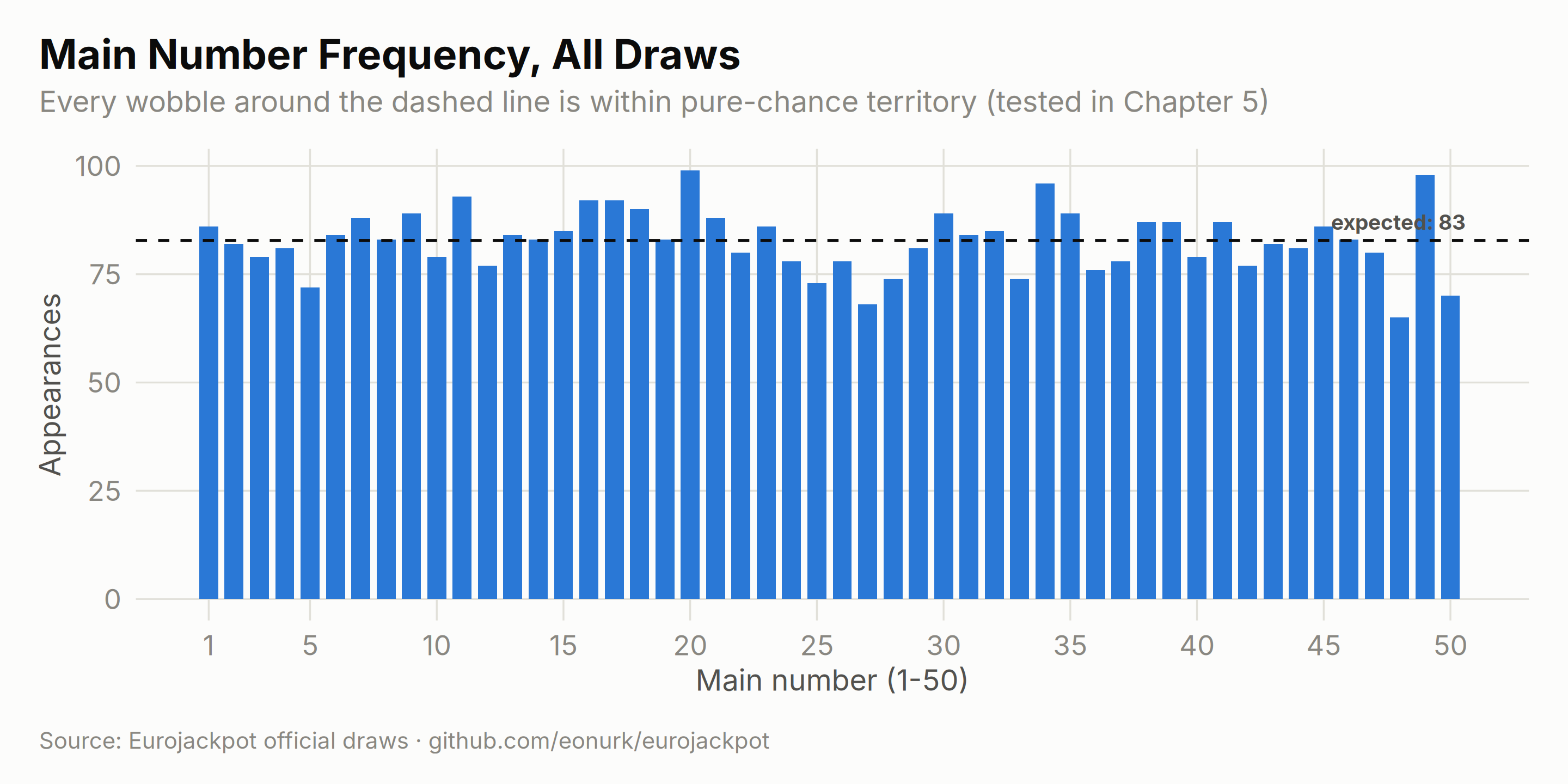
How often has each ball come out of the machine? For the main numbers a fair machine spreads appearances around 83 per number over the whole history:

main_freq_df <- data.frame(number = 1:50, frequency = tabulate(
    as.integer(as.matrix(results[, paste0("main_", 1:5)])),
    nbins = 50
))
expected_main <- 5 * n / 50

ggplot(main_freq_df, aes(x = number, y = frequency)) +
    geom_col(fill = ej_blue, width = 0.75) +
    geom_hline(yintercept = expected_main, linetype = "dashed", color = ej_ink, linewidth = 0.6) +
    annotate("text",
        x = 50.6, y = expected_main, label = sprintf("expected: %.0f", expected_main),
        hjust = 1, vjust = -0.7, size = 3.4, color = ej_ink2, fontface = "bold"
    ) +
    scale_x_continuous(breaks = c(1, seq(5, 50, by = 5))) +
    labs(
        title = "Main Number Frequency, All Draws",
        subtitle = "Every wobble around the dashed line is within pure-chance territory (tested in Chapter 5)",
        x = "Main number (1-50)", y = "Appearances", caption = ej_caption
    )

euro_freq_df <- data.frame(number = 1:12, frequency = tabulate(
    c(results$euro_1, results$euro_2),
    nbins = 12
))

ggplot(euro_freq_df, aes(x = number, y = frequency)) +
    geom_col(fill = ej_gold, width = 0.6) +
    scale_x_continuous(breaks = 1:12) +
    labs(
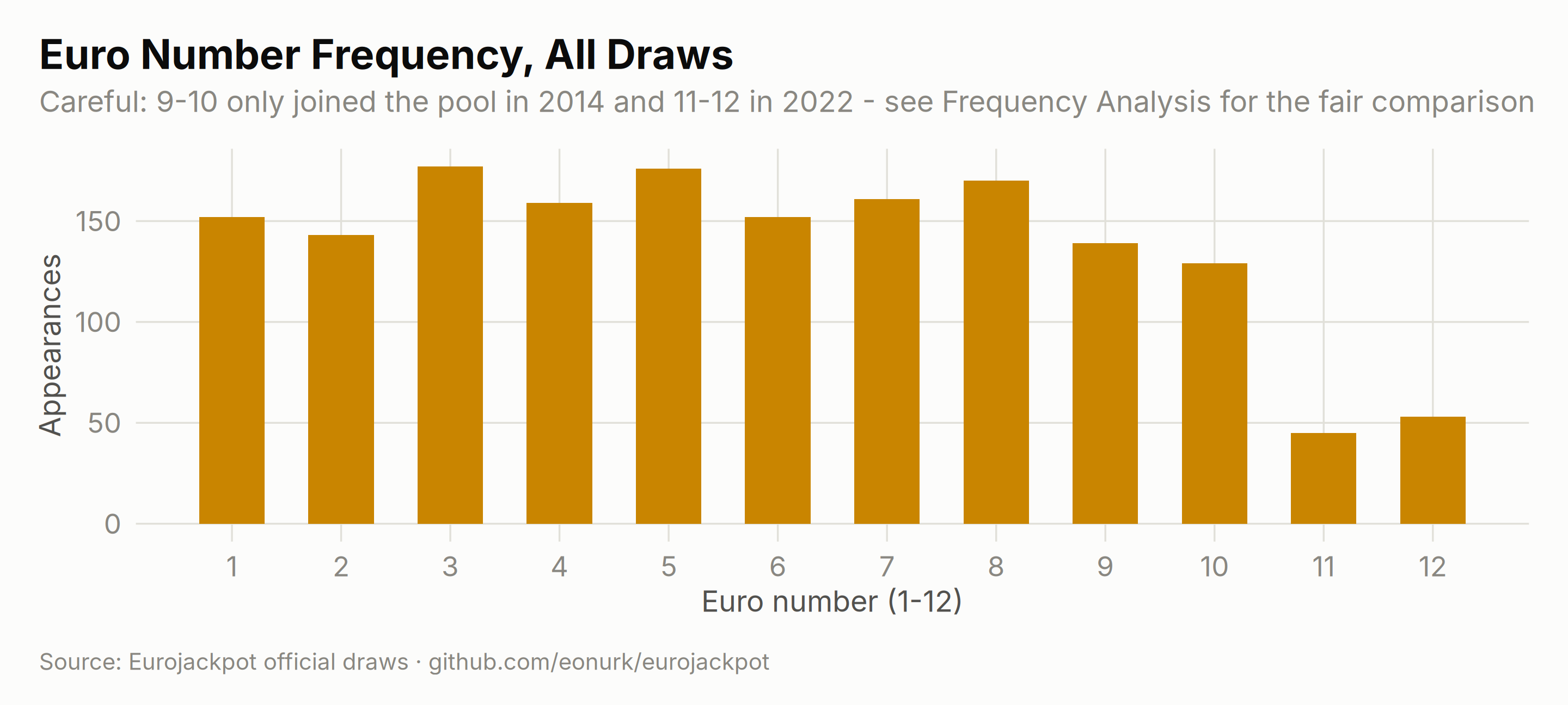
        title = "Euro Number Frequency, All Draws",
        subtitle = "Careful: 9-10 only joined the pool in 2014 and 11-12 in 2022 - see Frequency Analysis for the fair comparison",
        x = "Euro number (1-12)", y = "Appearances", caption = ej_caption
    )

4,140 main ballshave been drawn since 2012 — enough data to catch a biased machine, and exactly enough to show there isn’t one.

Pair Analysis

Which numbers like to travel together? With 1,225 possible main-number pairs and only 828 draws, even the “most frequent” pair is a rare guest:

# Function to count pairs of numbers
count_pairs <- function(data, columns) {
    pairs <- combn(columns, 2, function(cols) {
        pair_data <- data[, cols]
        return(paste(pair_data[, 1], pair_data[, 2], sep = "-"))
    }, simplify = FALSE)

    all_pairs <- unlist(pairs)
    pair_counts <- sort(table(all_pairs), decreasing = TRUE)
    return(pair_counts)
}

main_pairs <- count_pairs(results, paste0("main_", 1:5))
top_main_pairs <- head(main_pairs, 10)

top_pairs_df <- data.frame(
    pair = names(top_main_pairs),
    count = as.integer(top_main_pairs)
)

ggplot(top_pairs_df, aes(x = count, y = reorder(pair, count))) +
    geom_col(fill = ej_blue, width = 0.68) +
    geom_text(aes(label = count), hjust = -0.45, size = 3.3, color = ej_ink2, fontface = "bold") +
    scale_x_continuous(expand = expansion(mult = c(0, 0.1))) +
    labs(
        title = "Top 10 Main Number Pairs",
        subtitle = sprintf(
            "A random pair is expected together about %.1f times - the leaders are lucky, not magnetic",
            n * choose(5, 2) / choose(50, 2)
        ),
        x = "Times drawn together", y = NULL, caption = ej_caption
    ) +
    theme(panel.grid.major.y = element_blank())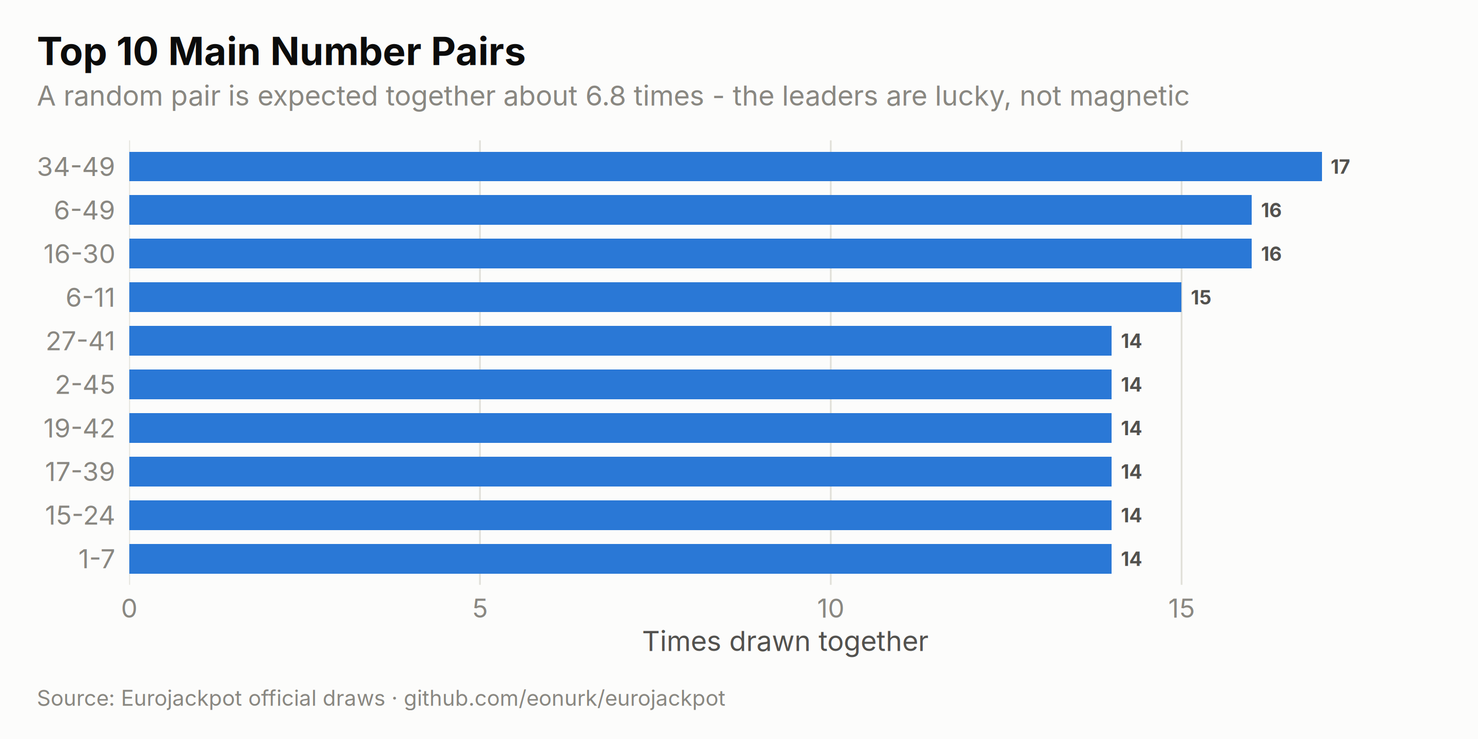

euro_pairs <- count_pairs(results, paste0("euro_", 1:2))
top_euro_pairs <- head(euro_pairs, 10)

euro_pairs_df <- data.frame(
    pair = names(top_euro_pairs),
    count = as.integer(top_euro_pairs)
)

ggplot(euro_pairs_df, aes(x = count, y = reorder(pair, count))) +
    geom_col(fill = ej_gold, width = 0.68) +
    geom_text(aes(label = count), hjust = -0.45, size = 3.3, color = ej_ink2, fontface = "bold") +
    scale_x_continuous(expand = expansion(mult = c(0, 0.1))) +
    labs(
        title = "Top 10 Euro Number Pairs",
        subtitle = sprintf("Out of %d euro pairs that have appeared at least once", length(euro_pairs)),
        x = "Times drawn together", y = NULL, caption = ej_caption
    ) +
    theme(panel.grid.major.y = element_blank())

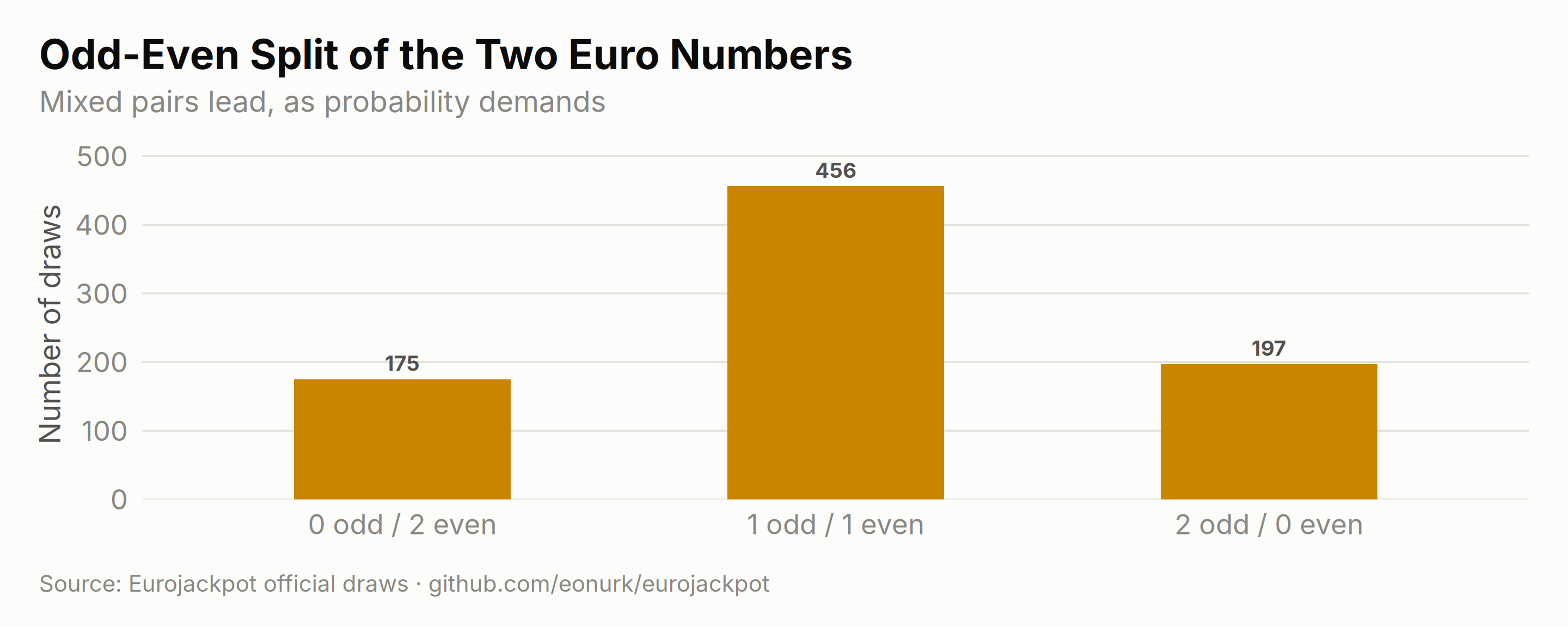
Odd-Even Distribution

Players love “balanced” tickets. The machine doesn’t care — but it does obey the hypergeometric distribution, which says a 3-2 or 2-3 odd-even split should dominate:

results$main_odd_count <- rowSums(results[, paste0("main_", 1:5)] %% 2 == 1)

odd_even_df <- data.frame(
    odd = 0:5,
    observed = as.integer(table(factor(results$main_odd_count, levels = 0:5))),
    expected = dhyper(0:5, 25, 25, 5) * n
)

ggplot(odd_even_df, aes(x = factor(odd))) +
    geom_col(aes(y = observed, fill = "Observed"), width = 0.66) +
    geom_point(aes(y = expected, color = "Expected (hypergeometric)"), size = 3.4) +
    scale_fill_manual(values = c("Observed" = ej_blue)) +
    scale_color_manual(values = c("Expected (hypergeometric)" = ej_ink2)) +
    scale_x_discrete(labels = paste0(0:5, " odd / ", 5:0, " even")) +
    labs(
        title = "Odd-Even Split of the Five Main Numbers",
        subtitle = "The machine matches textbook probability - \"balanced\" tickets are common because balance is common",
        x = NULL, y = "Number of draws", caption = ej_caption
    ) +
    theme(panel.grid.major.x = element_blank())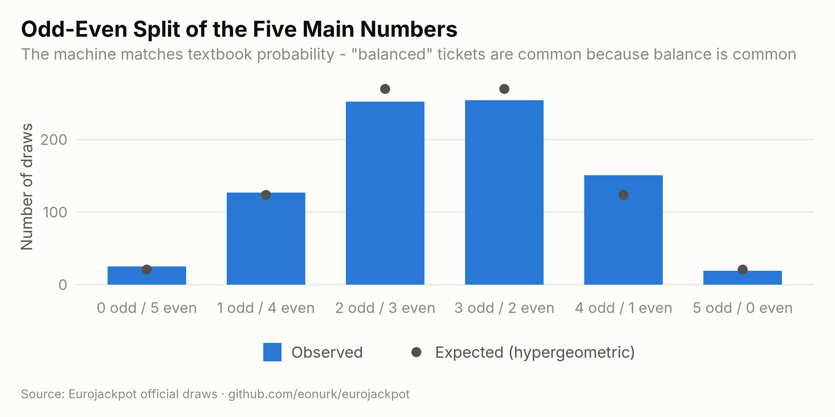

results$euro_odd_count <- rowSums(results[, paste0("euro_", 1:2)] %% 2 == 1)

euro_oe <- data.frame(
    odd = 0:2,
    observed = as.integer(table(factor(results$euro_odd_count, levels = 0:2)))
)

ggplot(euro_oe, aes(x = factor(odd), y = observed)) +
    geom_col(fill = ej_gold, width = 0.5) +
    geom_text(aes(label = observed), vjust = -0.55, size = 3.4, color = ej_ink2, fontface = "bold") +
    scale_x_discrete(labels = paste0(0:2, " odd / ", 2:0, " even")) +
    scale_y_continuous(expand = expansion(mult = c(0, 0.12))) +
    labs(
        title = "Odd-Even Split of the Two Euro Numbers",
        subtitle = "Mixed pairs lead, as probability demands",
        x = NULL, y = "Number of draws", caption = ej_caption
    ) +
    theme(panel.grid.major.x = element_blank())